Topology analysis
This vignette covers the basics of analyzing the topologies of Ig lineage
trees built using buildPhylipLineage, using some built-in alakazam functions
that focus on quantifying annotation relationships within lineages.
Example data
A small set of annotated example trees, ExampleTrees, are included in the alakazam package.
The trees are igraph objects with the following tree annotations (graph attributes):
clone: An identifier for the clonal group. These entries correspond to theclone_idcolumn in theExampleDbdata.frame from which the trees were generated.v_gene: IGHV gene name.j_gene: IGHJ gene name.junc_len: Length of the junction region (nucleotides).
And the following node annotations (vertex attributes):
sample_id: Time point in relation to influenza vaccination.c_call: The isotype(s) assigned to the sequence. Multiple isotypes are delimited by comma, and reflect identical V(D)J sequences observed with more than one isotype.duplicate_count: The copy number (duplicate count), which indicates the total number of reads with the same V(D)J sequence.
# Load required packages
library(alakazam)
library(igraph)
library(dplyr)

# Load example trees
data(ExampleTrees)

# Select one tree for example purposes
graph <- ExampleTrees[[24]]
# And add some annotation complexity to the tree
V(graph)$sample_id[c(2, 7)] <- "-1h"
V(graph)$c_call[c(2, 7)] <- "IGHM"

# Make a list of example trees excluding multi-isotype trees
graph_list <- ExampleTrees[sapply(ExampleTrees, function(x) !any(grepl(",", V(x)$c_call)))]
Plotting annotations on a tree
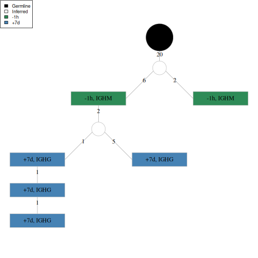
There are many options for configuring how an igraph object is plotted which are helpful for visualizing annotation topologies. Below is an extensive example of how to plot a tree by configuring the colors, labels, shapes and sizes of different visual elements according to annotations embedded in the graph.
# Set node colors
V(graph)$color[V(graph)$sample_id == "-1h"] <- "seagreen"
V(graph)$color[V(graph)$sample_id == "+7d"] <- "steelblue"
V(graph)$color[V(graph)$name == "Germline"] <- "black"
V(graph)$color[grepl("Inferred", V(graph)$name)] <- "white"

# Set node labels
V(graph)$label <- paste(V(graph)$sample_id, V(graph)$c_call, sep=", ")
V(graph)$label[V(graph)$name == "Germline"] <- ""
V(graph)$label[grepl("Inferred", V(graph)$name)] <- ""

# Set node shapes
V(graph)$shape <- "crectangle"
V(graph)$shape[V(graph)$name == "Germline"] <- "circle"
V(graph)$shape[grepl("Inferred", V(graph)$name)] <- "circle"

# Set node sizes
V(graph)$size <- 60
V(graph)$size[V(graph)$name == "Germline"] <- 30
V(graph)$size[grepl("Inferred", V(graph)$name)] <- 15

# Remove large default margins
par(mar=c(0, 0, 0, 0) + 0.05)

# Plot the example tree
plot(graph, layout=layout_as_tree, vertex.frame.color="grey",
     vertex.label.color="black", edge.label.color="black",
     edge.arrow.mode=0)

# Add legend
legend("topleft", c("Germline", "Inferred", "-1h", "+7d"),
       fill=c("black", "white", "seagreen", "steelblue"), cex=0.75)
Summarizing node properties
Various annotation dependent node statistics can be calculated using the
summarizeSubtrees and getPathLengths functions. getPathLengths
calculates distances from the root (germline) to child nodes, whereas
summarizeSubtrees calculates paths and subtree statistics
from child nodes.
Calculating distance from the germline
To determine the shortest path from the germline sequence to any node,
we use getPathLengths, which returns the distance both as the number
of “hops” (steps) and the number of mutational events (distance).
# Consider all nodes
getPathLengths(graph, root="Germline")
##             name steps distance
## 1      Inferred1     1       20
## 2 GN5SHBT04CW57C     2       26
## 3      Inferred2     3       28
## 4 GN5SHBT08I7RKL     4       29
## 5 GN5SHBT04CAVIG     5       30
## 6       Germline     0        0
## 7 GN5SHBT01D6X0W     2       22
## 8 GN5SHBT06H7TQD     6       31
## 9 GN5SHBT05HEG2J     4       33
Note, the STEPS counted in the above example include traversal of inferred
intermediates. If you want to exclude such nodes and consider only nodes
associated with observed sequences, you can specify an annotation field and
value that will be excluded from the number of steps. In the example below
we are excluding NA values in the c_call annotation
(field="c_call", exclude=NA).
# Exclude nodes without an isotype annotation from step count
getPathLengths(graph, root="Germline", field="c_call", exclude=NA)
##             name steps distance
## 1      Inferred1     0       20
## 2 GN5SHBT04CW57C     1       26
## 3      Inferred2     1       28
## 4 GN5SHBT08I7RKL     2       29
## 5 GN5SHBT04CAVIG     3       30
## 6       Germline     0        0
## 7 GN5SHBT01D6X0W     1       22
## 8 GN5SHBT06H7TQD     4       31
## 9 GN5SHBT05HEG2J     2       33
Note, steps has changed with respect to the previous example, but
distance remains the same.
Calculating subtree properties
The summarizeSubtrees function returns a table of each node with the
following properties for each node:
name: The node identifier.parent: The identifier of the node’s parent.outdegree: The number of edges leading from the node.size: The total number of nodes within the subtree rooted at the node.depth: The depth of the subtree that is rooted at the node.pathlength: The maximum path length beneath the node.outdegree_norm: Theoutdegreenormalized by the total number of edges.size_norm: Thesizenormalized by the total tree size.depth_norm: Thedepthnormalized by the total tree depth.pathlength_norm: Thepathlengthnormalized by the longest path.
The fields=c("sample_id", "c_call") argument in the example below simply
defines which annotations we wish to retain in the output. This argument
has no effect on the results, in constast to the behavior of getPathLengths.
# Summarize tree
df <- summarizeSubtrees(graph, fields=c("sample_id", "c_call"), root="Germline")
print(df[1:4])
##             name sample_id c_call         parent
## 1      Inferred1      <NA>   <NA>       Germline
## 2 GN5SHBT04CW57C       -1h   IGHM      Inferred1
## 3      Inferred2      <NA>   <NA> GN5SHBT04CW57C
## 4 GN5SHBT08I7RKL       +7d   IGHG      Inferred2
## 5 GN5SHBT04CAVIG       +7d   IGHG GN5SHBT08I7RKL
## 6       Germline      <NA>   <NA>           <NA>
## 7 GN5SHBT01D6X0W       -1h   IGHM      Inferred1
## 8 GN5SHBT06H7TQD       +7d   IGHG GN5SHBT04CAVIG
## 9 GN5SHBT05HEG2J       +7d   IGHG      Inferred2
print(df[c(1, 5:8)])
##             name outdegree size depth pathlength
## 1      Inferred1         2    8     6         13
## 2 GN5SHBT04CW57C         1    6     5          7
## 3      Inferred2         2    5     4          5
## 4 GN5SHBT08I7RKL         1    3     3          2
## 5 GN5SHBT04CAVIG         1    2     2          1
## 6       Germline         1    9     7         33
## 7 GN5SHBT01D6X0W         0    1     1          0
## 8 GN5SHBT06H7TQD         0    1     1          0
## 9 GN5SHBT05HEG2J         0    1     1          0
print(df[c(1, 9:12)])
##             name outdegree_norm size_norm depth_norm pathlength_norm
## 1      Inferred1          0.250 0.8888889  0.8571429      0.39393939
## 2 GN5SHBT04CW57C          0.125 0.6666667  0.7142857      0.21212121
## 3      Inferred2          0.250 0.5555556  0.5714286      0.15151515
## 4 GN5SHBT08I7RKL          0.125 0.3333333  0.4285714      0.06060606
## 5 GN5SHBT04CAVIG          0.125 0.2222222  0.2857143      0.03030303
## 6       Germline          0.125 1.0000000  1.0000000      1.00000000
## 7 GN5SHBT01D6X0W          0.000 0.1111111  0.1428571      0.00000000
## 8 GN5SHBT06H7TQD          0.000 0.1111111  0.1428571      0.00000000
## 9 GN5SHBT05HEG2J          0.000 0.1111111  0.1428571      0.00000000
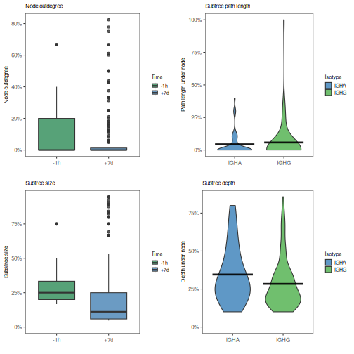
Distributions of normalized subtree statistics for a population of trees
can be plotted using the plotSubtrees function. In the example below,
we have specified silent=TRUE which causes plotSubtrees to return the
ggplot object without rendering the plot. The ggplot object are then
plotting using the gridPlot function which places each individual plot in
a separate panel of the same figure.
# Set sample colors
sample_colors <- c("-1h"="seagreen", "+7d"="steelblue")

# Box plots of node outdegree by sample
p1 <- plotSubtrees(graph_list, "sample_id", "outdegree", colors=sample_colors,
                   main_title="Node outdegree", legend_title="Time",
                   style="box", silent=TRUE)
# Box plots of subtree size by sample
p2 <- plotSubtrees(graph_list, "sample_id", "size", colors=sample_colors,
                   main_title="Subtree size", legend_title="Time",
                   style="box", silent=TRUE)
# Violin plots of subtree path length by isotype
p3 <- plotSubtrees(graph_list, "c_call", "pathlength", colors=IG_COLORS,
                   main_title="Subtree path length", legend_title="Isotype",
                   style="violin", silent=TRUE)
# Violin plots of subtree depth by isotype
p4 <- plotSubtrees(graph_list,  "c_call", "depth", colors=IG_COLORS,
                   main_title="Subtree depth", legend_title="Isotype",
                   style="violin", silent=TRUE)

# Plot in a 2x2 grid
gridPlot(p1, p2, p3, p4, ncol=2)
Counting and testing node annotation relationships
Given a set of annotated trees, you can determine the abundance of specific parent-child
relationships within individual trees using the tableEdges function and the
signficance of these relationships in population of trees using the testEdges
function. Annotation relationships over edges can be calculated as direct or indirect relationships, where a direct relationship is a parent-child pair and an indirect
relationship is a decent relationship that travels through another node (or nodes) first.
Tabulating edges for a single tree
Tabulating all directparent-child annotation relationships in the tree by isotype annotation can be performed like so:
# Count direct edges between isotypes
tableEdges(graph, "c_call")
## # A tibble: 5 × 3
## # Groups:   parent [3]
##   parent child count
##   <chr>  <chr> <int>
## 1 IGHG   IGHG      2
## 2 IGHM   <NA>      1
## 3 <NA>   IGHG      2
## 4 <NA>   IGHM      2
## 5 <NA>   <NA>      1
The above output is cluttered with the NA annotations from the germline and
inferred nodes. We can perform the same direct tabulation, but exclude any nodes
annotated with either Germline or NA for c_call using the exclude argument:
# Direct edges excluding germline and inferred nodes
tableEdges(graph, "c_call", exclude=c("Germline", NA))
## # A tibble: 1 × 3
## # Groups:   parent [1]
##   parent child count
##   <chr>  <chr> <int>
## 1 IGHG   IGHG      2
As there are inferred nodes in the tree, we might want to consider indirect
parent-child relationships that traverse through inferred nodes. This is accomplished
using the same arguments as above, but with the addition of the indirect=TRUE argument
which will skip over the excluded nodes when tabulating annotation pairs:
# Count indirect edges walking through germline and inferred nodes
tableEdges(graph, "c_call", indirect=TRUE, exclude=c("Germline", NA))
## # A tibble: 2 × 3
## # Groups:   parent [2]
##   parent child count
##   <chr>  <chr> <int>
## 1 IGHG   IGHG      2
## 2 IGHM   IGHG      2
Significance testing of edges in a population of trees
Given a population of trees, as a list of annotated igraph objects, you
can determine if there is enrichment for specific annotation pairs using the
testEdges function. This has the same options as tableEdges, except that
the values c("Germline", NA) are excluded by default. testEdges performs a
permutation test to generated a null distribution, excluding permutation of
of any annotations specified to the exclude argument (these annotation remain
fix in the tree). P-values output by testEdges are one-sided tests that the
annotation pair is observed more often than expected.
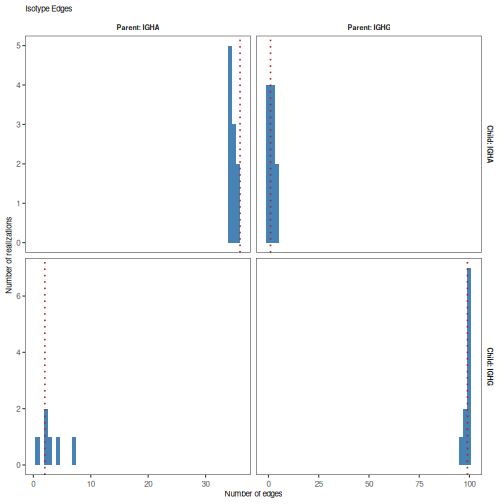
# Test isotype relationships
edge_test <- testEdges(graph_list, "c_call", nperm=10)

# Print p-value table
print(edge_test)
##   parent child count  expected pvalue
## 1   IGHA  IGHA    36 34.700000    0.0
## 2   IGHA  IGHG     2  3.166667    0.5
## 3   IGHG  IGHA     1  2.300000    0.6
## 4   IGHG  IGHG    99 99.100000    0.6
# Plot null distributions for each annotation pair
plotEdgeTest(edge_test, color="steelblue", main_title="Isotype Edges",
             style="hist")
Counting and testing MRCA annotations
The most recent common ancestor (MRCA) of an Ig lineage we define herein
as the most ancestral observed (or inferred) sequences in the lineage tree.
Meaning, the node that is most proximal (by some measure) to the germline/root
node. The getMRCA and testMRCA functions provide extraction and significance
testing of MRCA sequences by annotation value, respectively.
Extracting MRCAs from a tree
Extracting the MRCA from a tree is accomplished using the getMRCA function.
The germline distance criteria are as described above for getPathLengths
and can be either node hops or mutational events, with or without exclusion
of nodes with specific annotations. To simply extract the annotations for the
node(s) immediately below the germline, you can use the path=steps argument
without any node exclusion:
# Use unweighted path length and do not exclude any nodes
mrca_df <- getMRCA(graph, path="steps", root="Germline")

# Print subset of the annotation data.frame
print(mrca_df[c("name", "sample_id", "c_call", "steps", "distance")])
##                name sample_id c_call steps distance
## Inferred1 Inferred1      <NA>   <NA>     1       20
To use mutational distance and consider only observed (ie, non-germline and
non-inferred) nodes, we specify the exclusion field (field="c_call") and
exclusion value within that field (exclude=NA):
# Exclude nodes without an isotype annotation and use weighted path length
mrca_df <- getMRCA(graph, path="distance", root="Germline",
                   field="c_call", exclude=NA)

# Print excluding sequence, label, color, shape and size annotations
print(mrca_df[c("name", "sample_id", "c_call", "steps", "distance")])
##                          name sample_id c_call steps distance
## GN5SHBT01D6X0W GN5SHBT01D6X0W       -1h   IGHM     1       22
Significance testing of MRCA annotations
Similar to testEdges, the function testMRCA will perform a permutation
test to determine the significance of an annotation appearing at the MRCA
over a population of trees. P-values output by testMRCA are one-sided tests
that the annotation is observed more often than expected in the MRCA position.
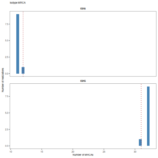
# Test isotype MRCA annotations
mrca_test <- testMRCA(graph_list, "c_call", nperm=10)
# Print p-value table
print(mrca_test)
##   annotation count expected pvalue
## 1       IGHA    12     11.1    0.0
## 2       IGHG    31     31.9    0.9
# Plot null distributions for each annotation
plotMRCATest(mrca_test, color="steelblue", main_title="Isotype MRCA",
             style="hist")