Amino acid property analysis
The alakazam package includes a set of functions to analyze the physicochemical
properties of Ig and TCR amino acid sequences. Of particular interest is the analysis of
CDR3 properties, which this vignette will demonstrate. The same process
can be applied to other regions simply by altering the sequence data column used.
Wu YC, et al. High-throughput immunoglobulin repertoire analysis distinguishes
    between human IgM memory and switched memory B-cell populations.
    Blood 116, 1070-8 (2010).
Wu YC, et al. The relationship between CD27 negative and positive B cell
    populations in human peripheral blood.
    Front Immunol 2, 1-12 (2011).
Example data
A small example AIRR database, ExampleDb, is included in the alakazam package.
# Load required packages
library(alakazam)
library(dplyr)

# Subset example data
data(ExampleDb)
db <- ExampleDb[ExampleDb$sample_id == "+7d", ]
For details about the AIRR format, visit the AIRR Community documentation site.
Calculate the properties of amino acid sequences
Multiple amino acid physicochemical properties can be obtained with the function
aminoAcidProperties. The available properties are:
length: total amino acid countgravy: grand average of hydrophobicitybulkiness: average bulkinesspolarity: average polarityaliphatic: normalized aliphatic indexcharge: normalized net chargeacidic: acidic side chain residue contentbasic: basic side chain residue contentaromatic: aromatic side chain content
This example demonstrates how to calculate all of the available amino acid
properties from DNA sequences found in the junction column of the previously loaded AIRR file.
Translation of the DNA sequences to amino acid sequences is accomplished by
default with the nt=TRUE argument. To reduce the junction sequence to the CDR3
sequence we specify the argument trim=TRUE which will strip the first and last
codon (the conserved residues) prior to analysis. The prefix cdr3 is added
to the output column names using the label="cdr3" argument.
db_props <- aminoAcidProperties(db, seq="junction", trim=TRUE,
                                label="cdr3")

# The full set of properties are calculated by default
dplyr::select(db_props[1:3, ], starts_with("cdr3"))
##   cdr3_aa_length cdr3_aa_gravy cdr3_aa_bulk cdr3_aa_aliphatic cdr3_aa_polarity
## 1             29     0.1724138     14.12345         0.8034483         8.168966
## 2             29    -0.3482759     14.69034         0.6724138         8.255172
## 3             26    -0.9884615     13.96154         0.5653846         8.873077
##   cdr3_aa_charge cdr3_aa_basic cdr3_aa_acidic cdr3_aa_aromatic
## 1     0.03902939     0.1034483     0.06896552       0.06896552
## 2     2.21407038     0.2068966     0.06896552       0.27586207
## 3     1.11045407     0.2307692     0.15384615       0.19230769
# Define a ggplot theme for all plots
tmp_theme <- theme_bw() + theme(legend.position="bottom")
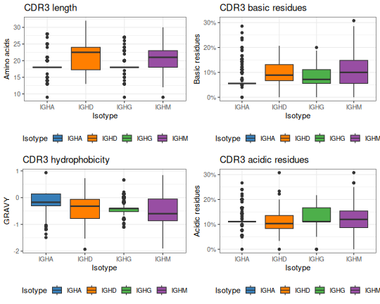
# Generate plots for all four of the properties
g1 <- ggplot(db_props, aes(x=c_call, y=cdr3_aa_length)) + tmp_theme +
ggtitle("CDR3 length") +
xlab("Isotype") + ylab("Amino acids") +
scale_fill_manual(name="Isotype", values=IG_COLORS) +
geom_boxplot(aes(fill=c_call))
g2 <- ggplot(db_props, aes(x=c_call, y=cdr3_aa_gravy)) + tmp_theme +
ggtitle("CDR3 hydrophobicity") +
xlab("Isotype") + ylab("GRAVY") +
scale_fill_manual(name="Isotype", values=IG_COLORS) +
geom_boxplot(aes(fill=c_call))
g3 <- ggplot(db_props, aes(x=c_call, y=cdr3_aa_basic)) + tmp_theme +
ggtitle("CDR3 basic residues") +
xlab("Isotype") + ylab("Basic residues") +
scale_y_continuous(labels=scales::percent) +
scale_fill_manual(name="Isotype", values=IG_COLORS) +
geom_boxplot(aes(fill=c_call))
g4 <- ggplot(db_props, aes(x=c_call, y=cdr3_aa_acidic)) + tmp_theme +
ggtitle("CDR3 acidic residues") +
xlab("Isotype") + ylab("Acidic residues") +
scale_y_continuous(labels=scales::percent) +
scale_fill_manual(name="Isotype", values=IG_COLORS) +
geom_boxplot(aes(fill=c_call))
# Plot in a 2x2 grid
gridPlot(g1, g2, g3, g4, ncol=2)
Obtaining properties individually
A subset of the properties may be calculated using the property argument of
aminoAcidProperties. For example, calculations may be restricted to only the
grand average of hydrophobicity (gravy) index and normalized net charge
(charge) by specifying property=c("gravy", "charge").
db_props <- aminoAcidProperties(db, seq="junction", property=c("gravy", "charge"),
                                trim=TRUE, label="cdr3")
dplyr::select(db_props[1:3, ], starts_with("cdr3"))
##   cdr3_aa_gravy cdr3_aa_charge
## 1     0.1724138     0.03902939
## 2    -0.3482759     2.21407038
## 3    -0.9884615     1.11045407
Using user defined scales
Each property has a default scale setting, but users may specify alternate scales
if they wish. The following example shows how to import and use the
Kidera et al, 1985 hydrophobicity scale and the Murrary et al, 2006 pK values from
the seqinr package instead of the defaults for calculating the GRAVY index and
net charge.
# Load the relevant data objects from the seqinr package
library(seqinr)
data(aaindex)
data(pK)
h <- aaindex[["KIDA850101"]]$I
p <- setNames(pK[["Murray"]], rownames(pK))
# Rename the hydrophobicity vector to use single-letter codes
names(h) <- translateStrings(names(h), ABBREV_AA)
db_props <- aminoAcidProperties(db, seq="junction", property=c("gravy", "charge"),
                                trim=TRUE, label="cdr3",
                                hydropathy=h, pK=p)
dplyr::select(db_props[1:3, ], starts_with("cdr3"))
##   cdr3_aa_gravy cdr3_aa_charge
## 1   -0.06551724     -0.0661116
## 2    0.10482759      2.0664863
## 3    0.13807692      1.0370349
Getting vectors of individual properties
The aminoAcidProperties function provides a convenient wrapper for calculating
multiple properties at once from a data.frame. If a vector of a specific property is
required this may be accomplished using one of the worker functions:
gravy: grand average of hydrophobicitybulk: average bulkinesspolar: average polarityaliphatic: aliphatic indexcharge: net chargecountPatterns: counts the occurrence of patterns in amino acid sequences
The input to each function must be a vector of amino acid sequences.
# Translate junction DNA sequences to amino acids and trim first and last codons
cdr3 <- translateDNA(db$junction[1:3], trim=TRUE)

# Grand average of hydrophobicity
gravy(cdr3)
## [1] 0.1724138 -0.3482759 -0.9884615
# Average bulkiness
bulk(cdr3)
## [1] 14.12345 14.69034 13.96154
# Average polarity
polar(cdr3)
## [1] 8.168966 8.255172 8.873077
# Normalized aliphatic index
aliphatic(cdr3)
## [1] 0.8034483 0.6724138 0.5653846
# Unnormalized aliphatic index
aliphatic(cdr3, normalize=FALSE)
## [1] 23.3 19.5 14.7
# Normalized net charge
charge(cdr3)
## [1] 0.03902939 2.21407038 1.11045407
# Unnormalized net charge
charge(cdr3, normalize=FALSE)
## [1] 0.03902939 2.21407038 1.11045407
# Count of acidic amino acids
# Takes a named list of regular expressions
countPatterns(cdr3, nt=FALSE, c(ACIDIC="[DE]"), label="cdr3")
##   cdr3_ACIDIC
## 1  0.06896552
## 2  0.06896552
## 3  0.15384615
Default scales
The following references were used for the default physicochemical scales:
- Aliphatic index:
Ikai AJ. Thermostability and aliphatic index of globular proteins. J Biochem 88, 1895-1898 (1980). - Bulkiness scale:
Zimmerman JM, Eliezer N, Simha R. The characterization of amino acid sequences in proteins by statistical methods. J Theor Biol 21, 170-201 (1968). - Hydrophobicity scale:
Kyte J, Doolittle RF. A simple method for displaying the hydropathic character of a protein. J Mol Biol 157, 105-32 (1982). - pK values:
\url{http://emboss.sourceforge.net/apps/cvs/emboss/apps/iep.html} - Polarity scale:
Grantham R. Amino acid difference formula to help explain protein evolution. Science 185, 862-864 (1974).